Quadratic Unconstrained Binary Optimization

Binary Quadratic Model

History

The Ising model is a classical model in statistical physics that describes the behavior of a collection of interacting magnetic spins. The spins can be in one of two states (up or down), and their interaction is described by a Hamiltonian that depends on the pairwise interactions between them. The goal is to find the configuration of spins that minimizes the energy of the system. Magnetic behavior can be understood by thinking of each atom as a spin, which can be pointing up or down:

\[\displaylines{ \begin{array}{|c|c|c|c|c|} \hline \color{blue}\uparrow & \color{blue}\uparrow & \color{red}\downarrow & \color{blue}\uparrow & \color{red}\downarrow \\ \hline \color{red}\downarrow & \color{blue}\uparrow & \color{blue}\uparrow & \color{red}\downarrow & \color{red}\downarrow \\ \hline \color{blue}\uparrow & \color{red}\downarrow & \color{blue}\uparrow & \color{blue}\uparrow & \color{red}\downarrow \\ \hline \color{red}\downarrow & \color{blue}\uparrow & \color{blue}\uparrow & \color{blue}\uparrow & \color{red}\downarrow \\ \hline \color{blue}\uparrow & \color{blue}\uparrow & \color{red}\downarrow & \color{red}\downarrow & \color{blue}\uparrow \\ \hline \end{array} }\]

Spins have a tendency to line up against or with a magnetic field’s direction. Neighboring spins influence each other, but not those further away. In order to represent these interactions we use linear terms for magnetic fields and pairwise quadratic for couplers. This is called the Ising Model where the energy (objective function) is defined as:

\[\displaylines{ \mathnormal{E} = - \sum_{i}{\mathnormal{h_i}\mathnormal{S_i} \ + \sum_{ij}{\mathnormal{J_{ij}S_iS_j}}} }\]

Where $\mathnormal{S}$ is spin which assumes the values:

\[\displaylines{ \mathnormal{S_i} \in \bigl\{-1, +1 \bigr\} }\]

$\mathnormal{h}$ and $\mathnormal{J}$ are adjustable constants. There is one $\mathnormal{h}$ for each spin and one $\mathnormal{J}$ for each interacting pair of spins.

Adiabatic Theorem in Quantum Computing

The adiabatic theorem is the foundation of a computational paradigm known as adiabatic quantum computation (AQC). The idea behind AQC is to exploit the adiabatic evolution of a quantum system to solve computational problems. This approach to ground state computation treats the entire energy landscape as a whole.

Here’s a high-level overview of how the adiabatic theorem is used in quantum computing:

Problem formulation: The computational problem is encoded into a Hamiltonian, which is a mathematical operator representing the energy of the quantum system. This Hamiltonian, known as the problem Hamiltonian, has a ground state (the lowest energy eigenstate) that corresponds to the solution of the problem.
Initialization: The quantum system is initialized in the ground state of a different Hamiltonian, called the initial Hamiltonian. This initial Hamiltonian is chosen such that its ground state is easy to prepare and is well-separated from the problem Hamiltonian.
Adiabatic evolution: The quantum system is evolved by slowly changing the Hamiltonian from the initial Hamiltonian to the problem Hamiltonian. According to the adiabatic theorem, if this change is sufficiently slow, the system will stay in the ground state throughout the evolution. At the end of this process, the system will be in the ground state of the problem Hamiltonian, which encodes the solution to the computational problem.
Measurement: The final state of the quantum system is measured, which yields the solution to the problem.

The main advantage of adiabatic quantum computing is that it does not rely on precise sequences of quantum gates, unlike the gate-model quantum computing. Instead, it uses the natural evolution of the quantum system to arrive at the desired final state. This can make adiabatic quantum computing more robust against certain types of errors and noise.

However, the adiabatic theorem imposes certain limitations on the speed of the computation. The Hamiltonian must be changed slowly enough to ensure that the system evolves adiabatically, which can potentially make the computation slower than other quantum computing methods. Additionally, the performance of AQC can be sensitive to the energy gap between the ground state and the first excited state of the Hamiltonian. If this gap becomes too small, the system may undergo non-adiabatic transitions, which can affect the accuracy of the computation.

QUBO

QUBO is ageneral optimization framework that can be used to solve a wide range of optimization problems, not just those related to spin systems. In QUBO, the problem is to minimize a quadratic objective function over binary variables (variables that can take on values of $0$ or $1$). The QUBO objective function can be written in terms of a matrix of coefficients, where the diagonal terms correspond to the linear terms, and the off-diagonal terms correspond to the quadratic terms.

\[Obj\mathnormal{(c, a_i, b_{ij}; q_i) = c + \sum_{i}{a_i q_i} + \sum_{i \lt j}{b_{ij} q_i q_j}}\]

$q$ are qubit variables $0$ and $1$ instead of $-1$ and $1$
$a$ and $b$ are adjustable constants

We can convert between $0/1$ variables and spins (Ising) via:

\[\displaylines{ \mathnormal{q_i} = \frac{1 + \mathnormal{S_i}}{2} }\]

QUBO can be used to solve the Ising model, and the Ising model can be formulated as a QUBO problem. Specifically, the QUBO objective function can be written to directly correspond to the energy function of the Ising model, where the binary variables in the QUBO problem correspond to the spin states in the Ising model.

QUBO provides a more general framework for optimization problems that includes the Ising model as a special case.

No division
Variables must be binary
There can be constants but is usually not written down
Triple products are not allowed
Support for linear and quadratic terms. Cubic or higher degrees are not allowed.
The constants do not affect the bitstring answers but affects the energy scale
The lowest energy solution is called the ground state
All solutions as a group is called an energy spectrum
A computation can return one or more solutions.

Examples of QUBOs

\[\displaylines{ \begin{array}{|l|l|} \hline \text{One-variable QUBO} &3\mathnormal{x} + 4\\ \hline \text{Two-variable QUBO} & 11 + 2.7\mathnormal{x} + 3\mathnormal{y} + 9.3\mathnormal{xy} \\ \hline \text{Three-variable QUBO} & \mathnormal{xy + xz - yz}\\ \hline \end{array} }\]

Not QUBOs

\[\displaylines{ \begin{array}{|l|l|} \hline \text{Cubic} &3\mathnormal{x} + 4 + \mathnormal{x}^3\\ \hline \text{Division} & 11 + 2.7\mathnormal{x} + 3\mathnormal{y} + 9.3\mathnormal{\frac{x}{y}} \\ \hline \text{Triple products} & \mathnormal{xyz}\\ \hline \end{array} }\]

Quantum Annealing Computers

Quantum Annealing Computers such as the D-Wave QPU solves QUBO or Ising Model problems. Quantum Machine Instructions in the form of a set of all the $a$ and $b$ values are sent to the QPU which finds the lowest-energy solution which results in the minimization of the objective function ($Obj$)

Graphical Representation of a QUBO

qubo_graph

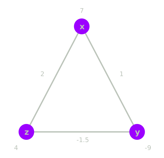
Quadratic terms appear on the edges.
Linear terms appear on the nodes.
Constant terms and variable names are usually ommitted but shown here.

\[\displaylines{ \mathcal{7x - 9y + 4z + xy + 2xz + 1.5yz} }\]

Represented as a matrix:

\[\displaylines{ \begin{bmatrix} 7 & 1 & 2\\ & -9 & -1.5\\ & & 4 \end{bmatrix} }\]

Binary Variables

Bbinary variables play a central role in QUBO, as they represent the choices and decisions in the combinatorial optimization problem. They are used to construct a quadratic objective function, which is then minimized to find the optimal solution to the problem.

Constraints are used to ensure that the solutions adhere to the requirements of the original combinatorial optimization problem. Constraints on binary variables can be expressed in various forms depending on the problem context. Here are some common types of constraints:

Mutually exclusive
Multiple choise
Conditional or contingent
Corequisite

Example Constraint

We use binary variables to express constraints for scheduling employees for a work shift. In these scenarios, let $x_i$, where $i$ is the employee number, represent whether an employee is selected for a work shift or not.

If the employee is not selected, then $x_i = 0$
If the employee is selected, then $x_i = 1$

Mutually Exclusive Constraints

One type of mutually exclusive constraint occurs when either one of two variables is a $1$. For example, a supervisor is not required for a work shift. But, if there is already one supervisor scheduled for a work shift, then another supervisor cannot be scheduled for that same shift. If employees number 1 and 2 are supervisors, this constraint can be expressed as the following inequality:

\[\displaylines{ \mathnormal{ x_1 + x_2 \le 1 }}\]

Which gives us the following truth table:

\[\displaylines{ \begin{array}{|c|c|c|c|} \hline x_1 & x_2 & x_1 + x_2 & \le 1 \ \text{(True/False)}\\ \hline 0 & 0 & 0 & \text{True}\\ \hline 1 & 0 & 1 & \text{True}\\ \hline 0 & 1 & 1 & \text{True}\\ \hline 1 & 1 & 2 & \text{False}\\ \hline \end{array} }\]

Multiple Choice Constraints

A multiple choice constraint occurs when only one variable can be a $1$. For example, now the company in our scenario requires exactly one supervisor per work shift. If employees number $1$ and $2$ are supervisors, this constraint can be expressed as the following inequality:

\[\displaylines{ \mathnormal{ x_1 + x_2 = 1 } }\]

Which gives us the following truth table:

\[\displaylines{ \begin{array}{|c|c|c|c|} \hline x_1 & x_2 & x_1 + x_2 & = 1 \ \text{(True/False)}\\ \hline 0 & 0 & 0 & \text{False}\\ \hline 1 & 0 & 1 & \text{True}\\ \hline 0 & 1 & 1 & \text{True}\\ \hline 1 & 1 & 2 & \text{False}\\ \hline \end{array} }\]

Conditional Constraints

A conditional (or sometimes called contingent) constraint occurs when one variable is dependent on another variable. For example, the company in our scenario requires that a supervisor in training must always be accompanied by a lead supervisor on a work shift. The lead supervisor can work a shift without the trainee. If employee number $3$ is a lead supervisor, and employee number $4$ is a trainee, then this constraint can be expressed as follows:

\[\displaylines{ \mathnormal{ x_4 \le x_3 } }\]

Which gives us the following truth table:

\[\displaylines{ \begin{array}{|c|c|c|c|} \hline x_3 & x_4 & x_4 \le x_3 & \text{(True/False)}\\ \hline 0 & 0 & \text{True} & \text{True}\\ \hline 1 & 0 & \text{False} & \text{False}\\ \hline 0 & 1 & \text{True} & \text{True}\\ \hline 1 & 1 & \text{True} & \text{True}\\ \hline \end{array} }\]

Corequisite Constraints

A corequisite constraint occurs when two or more variables must all be $1$. For example, the K-9 supervisor ($x_4$) must be on the same work shift as the search and rescue dog ($x_5$) or they cannot work. This constraint can be expressed as follows:

\[\displaylines{ x_4 = x_5 }\]

Which gives us the following truth table:

\[\displaylines{ \begin{array}{|c|c|c|c|} \hline x_4 & x_5 & x_4 = x_5 & \text{(True/False)}\\ \hline 0 & 0 & \text{True} & \text{True}\\ \hline 1 & 0 & \text{False} & \text{False}\\ \hline 0 & 1 & \text{False} & \text{False}\\ \hline 1 & 1 & \text{True} & \text{True}\\ \hline \end{array} }\]

Other Constraints

We can have a constraint where a specific variable must be $1$. In our example, we can use this for a situation where the K-9 supervisor must be selected for the work shift expressed as the following:

\[\displaylines{x_4 = 1}\]

We can have a constraint where either one of two variables must be $1$. In our example, either one of two specific employees or both must be selected for the work shift expressed as the following:

\[\displaylines{ x_1 + x_2 \ge 1 }\]

Which gives us the following truth table:

\[\displaylines{ \begin{array}{|c|c|c|c|} \hline x_1 & x_1 & x_1 + x_2 & \ge 1 \ \text{(True/False)}\\ \hline 0 & 0 & 0 & \text{False}\\ \hline 1 & 0 & 1 & \text{True}\\ \hline 0 & 1 & 1 & \text{True}\\ \hline 1 & 1 & 2 & \text{True}\\ \hline \end{array} }\]

We can have a constraint where an arbitrary number of variables in a set must be $1$ where in our example a maximum of $4$ employees from employees $1$ to $5$ can be selected for the work shift which we can express as the following:

\[\displaylines{ x_1 + x_2 + x_3 + x_4 + x_5 \le 4 }\]

If we want to have at least $3$ of the $4$ employees selected for the work shift:

\[\displaylines{ x_1 + x_2 + x_3 + x_4 \ge 3 }\] \[\]

Constraints with 3 Variables

We can extend the previous constraint type examples to use 3 variables. For our examples, we will use the same scenario of scheduling employees for a work shift. Let $x_i$ where $i$ is the employee number, represent whether an employee is selected for a work shift or not.

If the employee is not selected, then $x_i = 0$
If the employee is selected, then $x_i = 1$

Conditional Constraints

We can have a situation where we require that if employee $1$ is selected for the work shift, then employees $2$ and $3$ must also be selected. This conditional constraint is expressed and can be simplified as the following:

\[\displaylines{ x_1 \le x_2 \text{ and } x_1 \le x_3\\ 2x_1 - x_2 - x_3 \le 0 }\]

We can have a situation where we require that if employee $1$ is selected for a work shift, then employee $2$, employee $3$, or both must also be selected. Which we can express and simplify as the following:

\[\displaylines{ x_1 \le x_2 \text{ or } x_1 \le x_3\\ x_1 - x_2 - x_3 \le 0 }\]

We can have a situation where we require that if employees $2$ and $3$ are selected for a work shift, then employee $1$ must also be selected. Which we can express and simplify as the following:

\[\displaylines{ \text{If } x_2 + x_3 = 2, \text{ then } x_1 = 1\\ -x_1 + x_2 + x_3 \le 1 }\]

Mutually Exclusive Constraints with 3 variables

We can have a situation where we require that if employees $2$ and $3$ are both selected for a work shift, then employee $1$ cannot be selected. Which we can express and simplify as the following:

\[\displaylines{ \text{If } x_2 + x_3 = 2,\text{ then } x_1 = 0\\ x_1 + x_2 + x_3 \le 2 }\]

Simplifying Expressions

When working with binary variables, there is a helpful trick we can use to simplify expressions.

Since $0^2 = 0$ and $1^2 = 1$, we can replace any squared binary variable with an “unsquared” version. In other words $x^2 = x$

Multiplying Polynomials

When multiplying two polynomials, remember to multiplyeach term in the first polynomial by every term in the second. You may recall this as the FOIL method for binomials (two-term polynomials), which stands for First, Outside, Inside, Last.

\[\displaylines{ (-x^2 + 5)(-x + 5) = x^3 - 5x^2 - 5x + 25 }\]

To multiply trinomials, we multiplyeach term in one trinomial to each term in the other trinomial.

\[\displaylines{ \begin{align*} (x_1 + 2x_2 + 3x_3)(x_1 + x_2 + x_4) &= x_1(x_1 + x_2 + x_4) + 2x_2(x_1 + x_2 + x_4) + 3x_3(x_1 + x_2 + x_4)\\ &= x_1^2 + x_1 x_2 + x_1 x_4 + 2x_x x_2 + 2x_2^2 + 2x_2 x_4 + 3x_1 x_3 + 3x_2 x_3 + 3x_3 x_4\\ &= x_1^2 + 3x_1 x_2 + 3x_1 x_3 + x_1 x_4 + 2x_2^2 + 3x_2 x_3 + 2x_2 x_4 + 3x_3 x_4\\ \end{align*} }\]

To square polynomials using the form $\bigl(\sum{x_i}\bigr) - C$ where $C$ is some constant number we can use the general formula:

\[\displaylines{ \bigl(\bigl(\sum^{n}_{i=0}{x_i}\bigr) - C\bigr)^{2} = \bigl(\sum^{n}_{i=0}{x^2_i}\bigr) + 2 \bigl(\sum^{n}_{i=0}\sum^{n}_{j \gt i}{x_i x_j}\bigr) - 2C \bigl(\sum^{n}_{i = 0}{x_i}\bigr) + C^{2} }\]

Example QUBO Problem Minimization

\[\displaylines{ \text {Minimize } y = -5x_1 - 3x_2 - 8x_3 - 6x_4 + 4x_1 x_2 + 8x_1 x_3 + 2x_2 x_3 + 10x_3 x_4 }\]

First we isolate the linear terms and put it in a matrix:

\[\displaylines{ -5x_1 - 3x_2 - 8x_3 - 6x_4\\ \begin{bmatrix} -5 & & & \\ & -3 & & \\ & & -8 & \\ & & & -6 \\ \end{bmatrix} }\]

Then we can isolate the quadratic terms and insert them into the matrix:

\[\displaylines{ 4x_1 x_2 + 8x_1 x_3 + 2x_2 x_3 + 10x_3 x_4\\ \begin{bmatrix} -5 & 4 & 8 & 0\\ 0 & -3 & 2 & 0\\ 0 & 0 & -8 & 10\\ 0 & 0 & 0 & -6\\ \end{bmatrix} }\]

Example Two Qubit QUBO problems

Favor 2 qubits with the same value and penalize 2 qubits with different values

\[\displaylines{ \begin{array}{|c|c|c|} \hline x & y & ax + by + cxy + d\\ \hline 0 & 0 & 0 \\ \hline 0 & 1 & 1 \\ \hline 1 & 0 & 1 \\ \hline 1 & 1 & 0 \\ \hline \end{array} \\ Objective = x + y - 2xy }\]

We can use the solution “$+1, \ +1, \ -2$” where $a = +1, b = +1, c = -2, \text{ and } d = 0$

We want $x = 0 \text { and } y = 0$ and $x = 1 \text { and } y = 1$ to have the lowest values so that where both $x = y$ have the lowest energy state.
We assign the values as follows: $0 = d, 1 = b + d, 1 = a + d, 0 = a + b + c + d$
The values with the lowest number are called ground states and all possible values are called the spectrum

import dimod

exactsolver = dimod.ExactSolver()

Q = {(0, 0): 1, (1, 1): 1, (0, 1): -2}

results = exactsolver.sample_qubo(Q)

# print the results
for sample, energy in results.data(['sample', 'energy']):
    print(sample, energy)

{0: 0, 1: 0} 0.0
{0: 1, 1: 1} 0.0
{0: 1, 1: 0} 1.0
{0: 0, 1: 1} 1.0

Favor 2 qubits with different values and penalize 2 qubits with the same values

\[\displaylines{ \begin{array}{|c|c|c|} \hline x & y & ax + by + cxy + d\\ \hline 0 & 0 & 1 \\ \hline 0 & 1 & 0 \\ \hline 1 & 0 & 0 \\ \hline 1 & 1 & 1 \\ \hline \end{array} \\ Objective = 2xy - x - y + 1 }\]

We can use the solution “$-1, \ -1, \ +2$” where $a = -1, b = -1, c = +2, \text{ and } d = 1$
The ground states are where $x \ne y$
We assign the values as follows: $1 = d, 0 = b + d, 0 = a + d, 1 = a + b + c + d$
We use a constant $d = 1$ (energy offset) to ensure that the values have the same energies.

import dimod

exactsolver = dimod.ExactSolver()

Q = {(0, 0): -1, (1, 1): -1, (0, 1): 2}

results = exactsolver.sample_qubo(Q)

# print the results
for sample, energy in results.data(['sample', 'energy']):
    print(sample, energy)

{0: 1, 1: 0} -1.0
{0: 0, 1: 1} -1.0
{0: 0, 1: 0} 0.0
{0: 1, 1: 1} 0.0

Example Three Qubit Problem

\[\displaylines{ \begin{array}{|c|c|c|c|} \hline x & y & z & \text{Objective} \\ \hline 0 & 0 & 0 & 0\\ \hline 0 & 0 & 1 & 4\\ \hline 0 & 1 & 1 & -6.5\\ \hline 0 & 1 & 0 & -9\\ \hline 1 & 0 & 0 & 7\\ \hline 1 & 0 & 1 & 13\\ \hline 1 & 1 & 0 & -1\\ \hline 1 & 1 & 1 & 3.5\\ \hline \end{array} \\ Objective = 7x - 9y + 4z + xy + 2xz - 1.5yz }\]

The first excited state is $-6.5$ and the ground state is $-9$ which has a gap of $2.5$. Larger gaps result in better QPU performance.

Example QUBO Problems

Friends and Enemies

Given a set of people and information about some of their pairings being either a friend or an enemy.

graph LR
  xavier[Xavier] <-- Friends --> yolanda[Yolanda]
  yolanda <-- Enemies --> zeke[Zeke]
  zeke <-- Friends --> wanda[Wanda]

We can state our problem as follows:

Let $x =$ Xavier, $y =$ Yolanda, $z =$ Zeke, and $w =$ Wanda
Find qubit values ($0$ or $1$) such that: $x = y, y \ne z, z = w$

\[\displaylines{ \begin{array}{|c|c|c|} \hline x & 0 & \text{Xavier}\\ \hline y & 0 &\text{Yolanda}\\ \hline z & 1 & \text{Zeke}\\ \hline w & 1 &\text{Wanda}\\ \hline \end{array} }\]

We can represent this as a graph:

qubo_friends_enemies_graph

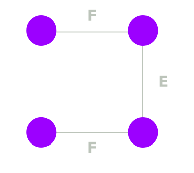
We want the lowest possible energy for $F$ (top and bottom) and $E$ such that

\[\displaylines{ \begin{align*} \text {Top pair of friends} &= F &= -1\\ \text {Bottom pair of friends} &= F &= -1\\ \text {Right pair of enemies} &= E &= -1\\ \hline & &= -3 \end{align*} }\]

A QUBO truth table for friends

\[\displaylines{ \begin{array}{|c|c|c|} \hline \text{Xavier} & \text{Yolanda} & ax+by+cxy+d\\ \hline 0 & 0 & -1\\ \hline 0 & 1 & 0\\ \hline 1 & 0 & 0\\ \hline 1 & 1 & -1\\ \hline \end{array} }\]

We can use the solution “$+1, \ +1, \ -2$” where $a = +1, b = +1, c = -2, \text{ and } d = -1$ constant to adjust the energy values which works out to $-1 = a + b + c + d$

A QUBO truth table for enemies

\[\displaylines{ \begin{array}{|c|c|c|} \hline \text{Yolanda} & \text{Zeke} & ey+fz+gyz+h\\ \hline 0 & 0 & 0\\ \hline 0 & 1 & -1\\ \hline 1 & 0 & -1\\ \hline 1 & 1 & 0\\ \hline \end{array} }\]

Here can use the solution “$-1, \ -1, \ +2$” where $e = -1, f = -1, g = +2, \text{ and } h = 0$ constant to adjust the energy values which works out to $0 = e + f + g + h$

Combining the sub-QUBOs produces the following graph:

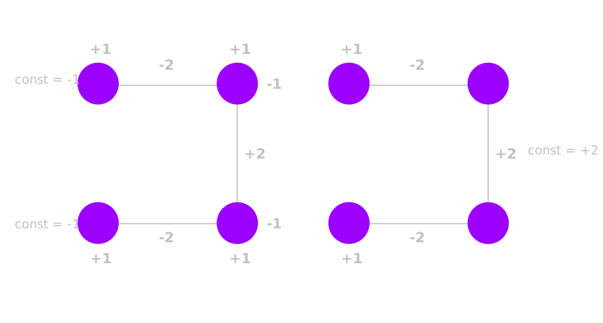
qubo_friends_enemies_graph_combined

Our truth table evaluation produces the following solutions in green:

\[\displaylines{ \begin{array}{|c|c|c|c|c|} \hline x & y & z & w & \text{objective}\\ \hline 0 & 0 & 0 & 0 & -2\\ \hline 0 & 0 & 0 & 1 & -1\\ \hline \color{green}0 & \color{green}0 & \color{green}1 & \color{green}0 & \color{green}-2\\ \hline \color{lime} 0 & \color{lime} 0 & \color{lime} 1 & \color{lime} 1 & \color{lime} -3\\ \hline 0 & 1 & 0 & 0 & -2\\ \hline 0 & 1 & 0 & 1 & -1\\ \hline 0 & 1 & 1 & 0 & 0\\ \hline 0 & 1 & 1 & 1 & -1\\ \hline \color{lime} 1 & \color{lime}1 & \color{lime}0 & \color{lime}0 & \color{lime}-3\\ \hline 1 & 1 & 0 & 1 & -2\\ \hline \end{array}\\ QUBO = -2 + x + w - 2xy + 2yz - 2zw }\]

Solution $\color{lime} (x = 0, y = 0, z = 1, w = 1)$
- Xavier and Yolanda are the same ✅
- Yolanda and Zeke are different ✅
- Zeke and Wanda are the same ✅
Solution $\color{lime} (x = 1, y = 1, z = 0, w = 0)$
- Xavier and Yolanda are the same ✅
- Yolanda and Zeke are different ✅
- Zeke and wanda are the same ✅

What if Xavier and Wanda are friends?

graph LR
  xavier[Xavier] <-- Friends --> yolanda[Yolanda]
  yolanda <-- Enemies --> zeke[Zeke]
  zeke <-- Friends --> wanda[Wanda]
  wanda <-- Friends --> xavier

We can express this algebraically as:

\[\displaylines{ \begin{align*} \text{x and y} &= -2xy + x + y - 1\\ \text{y and z} &= -y - z + 2yz\\ \text{z and w} &= -2zw + z + w - 1\\ \text{w and x} &= -2wx + w + x - 1\\ \text{QUBO} &= -2xy - 2xw + 2yz - 2zw + 2x + 2w - 3\\ \end{align*} }\]

Which produces the following table:

\[\displaylines{ \begin{array}{|c|c|c|c|c|} \hline x & y & z & w & \text{objective}\\ \hline 0 & 0 & 0 & 0 & -3\\ \hline 0 & 0 & 0 & 1 & -1\\ \hline \color{green}0 & \color{green}0 & \color{green}1 & \color{green}0 & \color{green}-3\\ \hline \color{lime} 0 & \color{lime} 0 & \color{lime} 1 & \color{lime} 1 & \color{lime} -3\\ \hline 0 & 1 & 0 & 0 & -3\\ \hline 0 & 1 & 0 & 1 & -1\\ \hline 0 & 1 & 1 & 0 & -1\\ \hline 0 & 1 & 1 & 1 & -1\\ \hline 1 & 0 & 0 & 0 & -1\\ \hline 1 & 0 & 0 & 1 & -1\\ \hline 1 & 0 & 1 & 0 & -1\\ \hline 1 & 0 & 1 & 1 & -3\\ \hline 1 & 1 & 0 & 0 & -3\\ \hline 1 & 1 & 0 & 1 & -3\\ \hline 1 & 1 & 1 & 0 & -1\\ \hline 1 & 1 & 1 & 1 & -3\\ \hline \end{array}\\ \text{QUBO} = -2xy - 2xw + 2yz - 2zw + 2x + 2w - 3\\ }\]

Solution $\color{lime}(x = 0, y = 0, z = 0, w = 0)$
- Xavier and Yolanda are the same ✅
- Yolanda and Zeke are the same ❌
- Zeke and Wanda are the same ✅
- Wanda and Xavier are the same ✅
Solution $\color{lime}(x = 0, y = 0, z = 1, w = 1)$
- Xavier and Yolanda are the same ✅
- Yolanda and Zeke are different ✅
- Zeke and Wanda are the same ✅
- Wanda and Xavier are different ❌

Another Friends and Enemies Problem

graph LR
  xavier[Xavier] <-- Friends --> yolanda[Yolanda]
  yolanda <-- Enemies --> zeke[Zeke]
  zeke <-- Friends --> cindy[Cindy]
  xavier <-- Friends --> wanda[Wanda]
  cindy <-- Enemies --> wanda

\[\displaylines{ \begin{array}{|c|c|c|c|c|c|} \hline & x & y & z & c & w\\ \hline x & 2 & -2 & 0 & 0 & -2\\ \hline y & 0 & 0 & 2 & 0 & 0\\ \hline z & 0 & 0 & 0 & -2 & 0\\ \hline c & 0 & 0 & 0 & 0 & 2\\ \hline w & 0 & 0 & 0 & 0 & 0\\ \hline \end{array} }\]

Jobs Problem

Suppose you have 5 jobs that need to be assigned to 3 workers. Each job has a certain difficulty level and each worker has a certain skill level. The goal is to minimize the total difficulty level of the jobs assigned to each worker, while ensuring that each worker is assigned exactly 2 jobs.

We can use binary variables to represent the assignment of jobs to workers. Specifically, we can use a binary variable $x_{ij}$ to represent whether job $i$ is assigned to worker $j$, where $i=1,2,3,4,5$ and $j=1,2,3$. If job $i$ is assigned to worker $j$, then $x_{ij}=1$, otherwise $x_{ij}=0$.

To minimize the total difficulty level of jobs assigned to each worker, we need to minimize the following objective function:

\[\displaylines{ \sum^5_{i=1} \sum^3_{j=1}{d_{i}x^2_{ij}} - \sum^3_{j=1}{s_j}\bigl(\sum^5_{i=1}{x_{ij} -2}\bigr)^2 }\]

where $d_i$ is the difficulty level of job $i$, $s_j$ is the skill level of worker $j$, and the first term penalizes assigning difficult jobs to workers, while the second term ensures that each worker is assigned exactly $2$ jobs.
We can express the objective function in terms of a QUBO matrix $Q$:

\[\displaylines{ \mathcal{Q} = \begin{bmatrix} d_{1} + s_{1} - 4d_{1}s_{1} & -2d_{1}s_{1} & -2d_{1}s_{3} & d_{1} & 0 & 0\\ -2d_{2}s_{1} & d_{2} + s_{2} - 4d_{2}s_{2} & -2d_{2}s_{3} & 0 & d_{2} & 0\\ -2d_{3}s_{1} & -2d_{3}s_{2} & d_{3} + s_{3} - 4d_{3}s_{3} & 0 & 0 & d_{3}\\ d_{1} & 0 & 0 & 0 & 0 &0\\ 0 & d_{2} & 0 & 0 & 0 & 0\\ 0 & 0 & d_{3} & 0 & 0 & 0\\ \end{bmatrix} }\]

The solution to the problem will be a set of binary variables that represent the optimal assignment of jobs to workers, where each worker has exactly 2 jobs and the total difficulty level of jobs assigned to each worker is minimized.